Base Class
MESH is written in an inheritance manner, so most of the functions in the base class can be directly accessed by subclasses. Usage of MESH involves writing a python script to call into various parts of MESH. Here we describe all of the MESH base class functions that can be called within the python environment.
For which functions can be called for a given geometry, please read the pages SimulationPlanar, SimulationGrating and SimulationPattern for the geometries you are simulating.
Note
The base class is just a wrapper for most of the functions, but it cannot be initiated in a python script. The only instances that can be initiated are the classes corresponding to different dimensions.
AddMaterial(material name, input file)
-
Arguments:
- material name: [string], the name of the material added to the simulation. Such name is unique and if there already exists a material with the same name, an error message will be printed out.
- input file: [string], a file that contains the dielectric properties of the corresponding material. For scalar dielectric, the input file should be formatted as a list of
omega eps_r eps_i
For diagonal dielectric, the format is a list of
omega eps_xx_r eps_xx_i eps_yy_r eps_yy_i eps_zz_r eps_zz_i
For tensor dielectric, the format is a list of
omega eps_xx_r eps_xx_i eps_xy_r eps_xy_i eps_yx_r eps_yx_i eps_yy_r eps_yy_i eps_zz_r eps_zz_i
-
Output: None
-
Note: The omega needs to be aligned for all the materials in the simulation.
AddMaterial(material name, omega, epsilon)
-
Arguments:
- material name: [string], the name of the material added to the simulation. Such name is unique and if there already exists a material with the same name, an error message will be printed out.
- omega: [tuple], all the omega values
- epsilon: [nested tuple], all the epsilon values
-
Output: None
-
Note: The omega needs to be aligned for all the materials in the simulation.
SetMaterial(material name, new epsilon)
-
Arguments:
- material name: [string], the name of the material whose epsilon will be changed. This material should already exist in the simulation (by
AddMaterial), otherwise an error will be printed out. - new epsilon: [nested tuple], the length equals the number of omega, and per row is the epsilon values with the same format as the input of
AddMaterialfunction. i.e. for scalar case the length will be , for diagonal case the length is and for tensor case the length is .
- material name: [string], the name of the material whose epsilon will be changed. This material should already exist in the simulation (by
-
Output: None
AddLayer(layer name, thickness, material name)
-
Arguments:
- layer name: [string], the name of the layer. Similarly, the names for layers are unique, and if such name already exists in the simulation, an error message will be printed out.
- thickness: [double], the thickness of the new layer in SI unit.
- material name: [string], the material that is used as the background of the layer. This material should already exist in the simulation (by
AddMaterial), otherwise an error message will be printed out.
-
Output: None
-
Note: this new added layer will be placed on top of all the previous layers.
SetLayer(layer name, thickness, material name)
-
Arguments:
- layer name: [string], the layer whose thickness and background will be changed. Such layer needs to already exist in the simulation, otherwise an error message will be printed out.
- thickness: [double], the new thickness of the layer.
- material name: [string], the material for the background of the layer. If such material does not exist, an error message will be printed out.
-
Output: None
SetLayerThickness(layer name, thickness)
-
Arguments:
- layer name: [string], the layer whose thickness will be changed. Such layer needs to already exist in the simulation, otherwise an error message will be printed out.
- thickness: [double], the new thickness of the layer.
-
Output: None
AddLayerCopy(new layer name, original layer name)
-
Arguments:
- new layer name: [string], the new layer that is copied from the original layer. Such name cannot already exist in the simulation, otherwise an error message will be printed out.
- original layer name: [string], the original layer from whom everything is copied. If this layer does not exist in the simulation, an error will be printed out.
-
Output: None
-
Note: this function only copies the structure information, for example any pattern of the original layer, but does not copy any thermal information. For example, even the original layer is set as a source, the copied layer is still not a source. In addition, this new added layer will be placed on top of all the previous layers.
DeleteLayer(layer name)
-
Arguments:
- layer name: [string], the name of the layer that will be deleted. Such layer should already be in the system, otherwise an error will be printed out.
-
Output: None
SetSourceLayer(layer name)
-
Arguments:
- layer name: [string], the name of the layer that is designated as the source layer. Such layer should already exist in the system, otherwise an error will be printed out.
-
Output: None
-
Note: a system can have more than source layers.
SetProbeLayer(layer name)
-
Arguments:
- layer name: [string], the name of the layer that is designated as the probe layer of the flux. Such layer should already exist in the system, otherwise an error will be printed out.
-
Output: None
-
Note: a system can have only one probe layer. Setting another layer as the probe layer will overwrite the previous one. In addition, the probe layer should be above all the source layers in the real geometry.
SetProbeLayerZCoordinate(target_z)
-
Arguments:
- target_z: [double], the zth coordinate in the target layer where the Poynting flux is evaluated. By default this value is the thickness of the target layer
-
Output: None
SetThread(nthread)
-
Arguments:
- nthreads: [int], number of threads used in OpenMP.
-
Output: None
- Note: this function only works in an OpenMP setup.
SetKxIntegral(points, end)
-
Arguments:
- points: [int], number of points in the integration.
- end: [double, optional for grating and pattern geometries], the end of the integral over . This end should be a normalized number with respect to .
-
Output: None
-
Note: this function is essentially doing where the integral is evaluated as a summation of
pointspoints. In the case whenendis not given, the lower and upper bounds of the integral will be . where is the length of the reciprocal lattice with component in direction. See the following figure: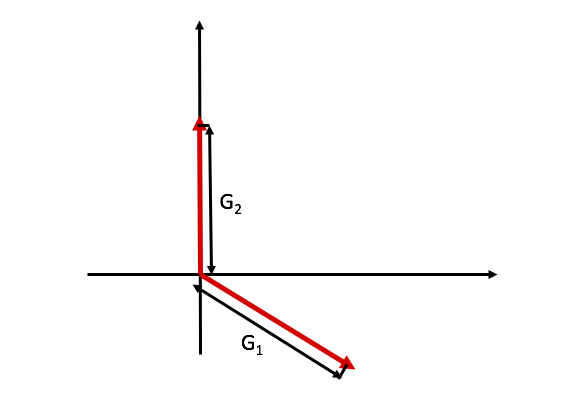
SetKyIntegral(points, end)
-
Arguments:
- points: [int], number of points in the integration.
- end: [double, optional for pattern geometries], the end of the integral over . This end should be a normalized number with respect to .
-
Output: None
-
Note: this function is essentially doing where the integral is evaluated as a summation of
pointspoints. In the case whenendis not given, the lower and upper bounds of the integral will be , where is the length of the reciprocal lattice along direction
SetKxIntegralSym(points, end)
-
Arguments:
- points: [int], number of points in the integration.
- end: [double, optional for grating and pattern geometries], the end of the integral over . This end should be a normalized number with respect to .
-
Output: None
-
Note: this function is essentially doing where the integral is evaluated as a summation of
pointspoints. In the case whenendis not given, the upper bound of the integral will be .
SetKyIntegralSym(points, end)
-
Arguments:
- points: [int], number of points in the integration.
- end: [double, optional for pattern geometries], the end of the integral over . This end should be a normalized number with respect to .
-
Output: None
-
Note: this function is essentially doing where the integral is evaluated as a summation of
pointspoints. In the case whenendis not given, the upper bound of the integral will be .
InitSimulation()
-
Arguments: None
-
Note: this function builds up the structure of the system.
IntegrateKxKy()
-
Arguments: None
-
Output: None
-
Note: this function integrates over and based on the integral properties set by the user. So the function can only be called after the and integrals are configured, and the system is initialized.
IntegrateKxKyMPI(rank, size)
-
Arguments:
- rank: [int], the rank of the thread.
- size: [int], the total size of the MPI run.
-
Output: None
-
Note: this function can only be called during MPI. For an example of a funtion call, please refer to MPI example.
GetNumOfOmega()
-
Arguments: None
-
Output: [int], the number of total omega points computed in the simulation.
GetPhi()
-
Arguments: None
-
Output: [tuple of double], the values obtained from the simulation.
-
Note: can only be called after and are integrated.
GetOmega()
-
Arguments: None
-
Output: [tuple of double], the omega values computed in the simulation.
GetEpsilon(omega index, (x, y, z))
-
Arguments:
- omega index: [int], the index of the omega value where is evaluated. To be consistent with python, this index starts from .
- (x, y, z): [double tuple], the real space position where the index is evaluated, in SI unit
-
Output: value of epsilon with length , in the form of
eps_xx_r, eps_xx_i, eps_xy_r, eps_xy_i, eps_yx_r, eps_yx_i, eps_yy_r, eps_yy_i, eps_zz_r, eps_zz_iThese are computed by reconstruction of the Fourier series, so won't be the same as the exact dielectric function.
GetPhiAtKxKy(omega index, kx, ky)
-
Arguments:
- omega index: [int], the index of the omega value where is evaluated. To be consistent with python, this index starts from .
- kx: [double], the value where is evaluated. It is a normalized value by .
- ky: [double], the value where is evaluated. It is a normalized value by .
-
Output: [double], the value of .
OutputSysInfo()
-
Arguments: None
-
Output: None
-
Note: the function prints out a system description to screen.
OutputLayerPatternRealization(omega index, name, Nu, Nv, filename)
-
Arguments:
- omega index: [int], the index of the omega value that the dielectric is evaluated. To be consistent with python, this index starts from .
- name: [string], the name of the layer.
- Nu: [int], number of points in x direction in one periodicity.
- Nv: [int], number of points in y direction in one periodicity.
- filename: [string], optional. If not given, then the epsilon values will be printed to standard output.
-
Output: None
-
Note: the epsilon format will be the same as the function
GetEpsilonalong with the spacial coordinates.
Also, MESH provides some options for printing intermediate information and methods for Fourier transform of the dielectric.
OptOnlyComputeTE()
-
Arguments: None
-
Output: None
-
Note: with this function, the package only computes flux contributed from TE mode.
OptOnlyComputeTM()
-
Arguments: None
-
Output: None
-
Note: with this function, the package only computes flux contributed from TM mode.
OptPrintIntermediate(output_flag)
-
Arguments:
- output_flag [string, optional], the output file suffix.
-
Output: None
-
Note: this function prints intermediate to file when function
IntegrateKxKy()orIntegrateKxKyMPI(rank, size)is called. The output format is a list of " ", where and are values normalized to .
MESH provides class for linear interpolating data points. In Python, the class can be initiated using
from MESH import Interpolator
interpolator = Interpolator(data)
-
Arguments:
- data: [nested tuples], in the form of ( (, )...(, )), where should also be a tuple.
-
Output: None
At a certain point , the interpolated can be retrieved by
interpolator.Get(x)
-
Arguments:
- x: [double], the point where the interpolation is performned
-
Output: a tuple of values at
MESH also provides physics constants to facilitate computation. The constant object can be initiated by
from MESH import Constants
constant = Constants()
The supported constants are (all in SI unit)
- constant['pi']: the value of .
- constant['k_B']: the value of .
- constant['eps_0']: the value of .
- constant['mu_0']: the value of .
- constant['m_e']: the value of , i.e. the mass of an electron.
- constant['eV']: electron volt in Joules.
- constant['h']: the value of Planck's constant.
- constant['h_bar']: the value of the reduced Planck's constant.
- constant['c_0']: the speed of light.
- constant['q']: the value of , i.e. magnitude of electron charge.
- constant['sigma']: the value of , i.e. Stefan-Boltzmann constant.